Human tooth | Homo

We recently were able to publish a study where we automatically segmented the root canal space in human teeth: doi:10.1186/s12903-021-01551-x

Here’s a little explanation of the study, in which we used the sample changer of our SkyScan 1272 quite intensively. In collaboration with the zmk bern – Zahnmedizinische Kliniken we were asked to image +100 human teeth (excess material from tooth operations/extractions) and prepare the tomographic datasets for characterization. As mentioned, we used the sample changer of our scanner for this, on which we mounted each tooth in a custom-designed and 3D-printed sample holder. After aqcuiring +800 GB of raw data we reconstructed the data into about 350 GB of reconstructions. All these reconstructions were then ingested into a pipeline in a Jupyter notebook with Python code. The notebook is freely available here: https://github.com/habi/zmk-tooth-cohort and is able to be run with binder by clicking the relevant button in the GitHub repository above.

After we’ve prepared the data for our collaborators we’ve tried to write up the whole process as a publication. This was achieved by using the collaborative writing function of Manuscripts.io. A ready to submit-version of the manuscript was exported to a set of Markdown files and imported into a manubot-enabled repository on GitHub, which automatically converts the text into both a nice-looking website and PDF file.

The tooth shown in the header image of this post was scanned on a SkyScan 1272 with a source voltage of 80 kV, a source current of 125 µA with camera and geometry settings leading to an isotropic voxel size of 10 µm. The whole scan of this tooth took about 3 hours and 15 minutes. The animation was generated with MeVisLab using the MeVis Path Tracer feature. The movie was generated from a set of single frames in the same manner as described previously.

Lecture on (micro)tomography

Today, I gave a lecture on (micro)tomography, in front of a bunch of students from the University of Bern, as part of the Lecture Series on Advanced Microscopy. I tried to show them what can be nicely done with - for example - our desktop micro-CT scanners. The whole presentation was crafted in LaTeX and is available on GitHub, should you be interested in it. The student handout of the presentation was automatically compiled and put online using a GitHub Action (this one here), you can download a copy of the handout here if you like.

The poster image of this blog post shows a three-dimensional visualization of a mouse skull which is approximately 25 mm long from the nose to the back of the skull. The mouse head was scanned on a SkyScan 1172 with a source voltage of 59 kV, a source current of 167 µA with camera and geometry settings leading to an isotropic voxel size of 7.96 µm. The whole scan took about 74 minutes. I used the data set throughout the lecture to show different details and intricacies of the tomographic imaging process.

The data set was visualized in MeVisLab with the MeVis Path Tracer feature. The movie was generated from a set of single frames in the same manner as described previously.

Adaptation of zebrafish gills to endurance training

As mentioned before, we’ve been working with a bunch of Zebrafishes lately. For a project on the adaptation of zebrafish gills to endurance training we have been performing a part of the tomographic imaging (the details are specified in the liked post above) as well as the in-depth analysis of the data.

The result of the whole project has recently been accepted as a peer-reviewed manuscript at PLOS ONE. You can find the published version here at doi:10.1371/journal.pone.0228333. Earlier, we submitted a non-peer-reviewed version to bioRxiv which can be found here at doi:10.1101/744300.

A quick rundown on how we got to the results:

• One group of fishes was trained in a swim tunnel, they trained relatively to an Olympic athlete, a control group was lazily swimming in a turned-off swim tunnel.
• After training (or non-training), the fishes were sacrificed and prepared for tomographic imaging by our expert lab technicians.
• Oleksiy, Fluri and me scanned the fishes on our old and trusty SkyScan 1172.
• Dea and Matthias delineated the gills in the tomographic datasets, which was the basis for our analysis (the delineated regions are made available by the OSF).
• In a Jupyter we ingested all the data, scattered over the delineated tomographic datasets and several XLS files from the collaborators (the Jupyter notebook is available on GitHub here).
• Based on the measured data we were (among other things) able to show that the gills of trained zebrafish appear significantly more sparse (p=0.0088) than the control group. In our opinion, this means that the water can penetrate the gills and pass the gills much more easily in the trained fishes, e.g. they can ‘breathe’ more easily after a certain training period.
• All the other results, including oxygen consumption and mitoses on the tips of the gills are in themselves also interesting, but have not been performed by me.

Should you be interested in taking a look at how we got to the results, you find the complete analysis (in a Jupyter notebook) and a link to the tomographic datasets of the delineated gills here at GitHub.

Mouse lung | Mus

In a new project we scan mouse lungs in which tumors were induced. The lung was critically-point-dried and scanned on a SkyScan 1272 with a source voltage of 50 kV, a source current of 200 µA with camera and geometry settings leading to an isotropic voxel size of 8 µm. The whole scan took about 53 minutes. The tumor is visible in the lower part of the left lung lobe and has a size of approximately 2 mm.

The data set was visualized in CTVox and exported to a set of images. We manually removed some cruft in the images and generated a movie as described before.

Zebrafish gills | Danio rerio

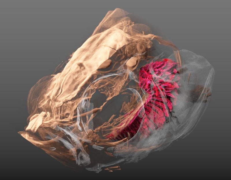
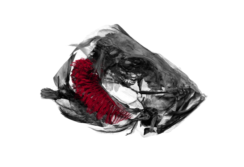
For a recent project (hopefully more to follow soon) we needed to visualize the head of a zebrafish with its gills inside. The image above shows a three-dimensional visualization of a tomographic scan of such a head, critically point dried. After drying, the head was scanned on a SkyScan 1172 with a source voltage of 50 kV, a source current of 167 µA with camera and geometry settings leading to an isotropic voxel size of 1.65 µm, the scan took several hours.

The left part of the head is rendered semi-transparently so that the (manually delineated) gills are nicely visible in red. The tip-to-tip distance of the gills (shown in red) is approximately 1.9 mm.

The data set was visualized in MeVisLab with the MeVis Path Tracer feature.